Post-workshop exercises

Optional exercises to test your knowledge and reinforce your learning

Prep

Have the dplyr, tidyr, and ggplot cheatsheets ready open and ready.

Load packages

the code below will load the packages you need:

library(tidyverse)
library(car)

Load datasets

The code below will load and print the first few rows of the Duncan dataset. To find out more about this dataset, type ?Duncan in your RStudio console to open the vignette.

duncan <- as_tibble(Duncan)
print(duncan)

# A tibble: 45 × 4
   type  income education prestige
   <fct>  <int>     <int>    <int>
 1 prof      62        86       82
 2 prof      72        76       83
 3 prof      75        92       90
 4 prof      55        90       76
 5 prof      64        86       90
 6 prof      21        84       87
 7 prof      64        93       93
 8 prof      80       100       90
 9 wc        67        87       52
10 prof      72        86       88
# ℹ 35 more rows

The code below will load and print the first few rows of the WVS dataset. To find out more about this dataset, type ?WVS in your RStudio console to open the vignette.

wvs <- as_tibble(WVS)
print(wvs)

# A tibble: 5,381 × 6
   poverty     religion degree country   age gender
   <ord>       <fct>    <fct>  <fct>   <int> <fct> 
 1 Too Little  yes      no     USA        44 male  
 2 About Right yes      no     USA        40 female
 3 Too Little  yes      no     USA        36 female
 4 Too Much    yes      yes    USA        25 female
 5 Too Little  yes      yes    USA        39 male  
 6 About Right yes      no     USA        80 female
 7 Too Much    yes      no     USA        48 female
 8 Too Little  yes      no     USA        32 male  
 9 Too Little  yes      no     USA        74 female
10 Too Little  yes      no     USA        30 male  
# ℹ 5,371 more rows

Question 1

Using wvs dataset, filter the age column to include values that is more than 29. Then, select the columns age, degree, religion and poverty. Save the result to a new dataframe called wvs_filtered.

Show Answer

wvs_filtered <- wvs |> 
    filter(age > 29) |> 
    select(age, degree, religion, poverty) 

print(wvs_filtered)

# A tibble: 4,228 × 4
     age degree religion poverty    
   <int> <fct>  <fct>    <ord>      
 1    44 no     yes      Too Little 
 2    40 no     yes      About Right
 3    36 no     yes      Too Little 
 4    39 yes    yes      Too Little 
 5    80 no     yes      About Right
 6    48 no     yes      Too Much   
 7    32 no     yes      Too Little 
 8    74 no     yes      Too Little 
 9    30 no     yes      Too Little 
10    32 yes    yes      Too Little 
# ℹ 4,218 more rows

Question 2

Update the wvs dataset by creating a dummy-coded version of the gender variable, where male = 0 and female = 1. Save the results in a new column named gender_coded.

Show Answer

wvs <- wvs |> 
    mutate(gender_coded = if_else(gender == "male", 0, 1)) 

print(wvs)

# A tibble: 5,381 × 7
   poverty     religion degree country   age gender gender_coded
   <ord>       <fct>    <fct>  <fct>   <int> <fct>         <dbl>
 1 Too Little  yes      no     USA        44 male              0
 2 About Right yes      no     USA        40 female            1
 3 Too Little  yes      no     USA        36 female            1
 4 Too Much    yes      yes    USA        25 female            1
 5 Too Little  yes      yes    USA        39 male              0
 6 About Right yes      no     USA        80 female            1
 7 Too Much    yes      no     USA        48 female            1
 8 Too Little  yes      no     USA        32 male              0
 9 Too Little  yes      no     USA        74 female            1
10 Too Little  yes      no     USA        30 male              0
# ℹ 5,371 more rows

Question 3

Create a summary of the wvs dataset showing the number of observations for each country.

Show Answer

wvs |> 
    count(country)

# A tibble: 4 × 2
  country       n
  <fct>     <int>
1 Australia  1874
2 Norway     1127
3 Sweden     1003
4 USA        1377

Question 4

Using wvs dataset, calculate the average age for each combination of gender and degree status.

Show Answer

wvs |> 
    group_by(gender, degree) |> 
    summarise(avg_age = mean(age, na.rm = TRUE))

`summarise()` has grouped output by 'gender'. You can override using the
`.groups` argument.

# A tibble: 4 × 3
# Groups:   gender [2]
  gender degree avg_age
  <fct>  <fct>    <dbl>
1 female no        45.6
2 female yes       41.0
3 male   no        46.0
4 male   yes       43.3

Question 5

Using the wvs dataset, create a summary statistics for each country and religion (yes/no). Calculate the age mean, age median, number of observation.

Show Answer

wvs |> 
    group_by(country, religion) %>%
    summarise(
        avg_age = mean(age, na.rm = TRUE),
        median_age = median(age, na.rm = TRUE),
        n_observations = n()
    )

`summarise()` has grouped output by 'country'. You can override using the
`.groups` argument.

# A tibble: 8 × 5
# Groups:   country [4]
  country   religion avg_age median_age n_observations
  <fct>     <fct>      <dbl>      <dbl>          <int>
1 Australia no          39.9         37            375
2 Australia yes         45.7         43           1499
3 Norway    no          40.6         38            109
4 Norway    yes         43.6         42           1018
5 Sweden    no          43.7         42             15
6 Sweden    yes         43.9         43            988
7 USA       no          44.6         42            287
8 USA       yes         48.9         46           1090

Question 6

Using the wvs dataset, select the 10 oldest respondents from the USA. (hint: arrange() and slice())

Show Answer

wvs |> 
    filter(country == "USA", age > 50) |> 
    arrange(desc(age)) |> 
    slice(1:10)

# A tibble: 10 × 7
   poverty     religion degree country   age gender gender_coded
   <ord>       <fct>    <fct>  <fct>   <int> <fct>         <dbl>
 1 Too Much    no       no     USA        91 male              0
 2 Too Little  yes      no     USA        91 male              0
 3 Too Much    yes      no     USA        88 female            1
 4 About Right yes      no     USA        88 male              0
 5 Too Little  yes      yes    USA        87 female            1
 6 Too Much    yes      no     USA        87 female            1
 7 Too Little  yes      no     USA        87 male              0
 8 About Right yes      no     USA        87 male              0
 9 About Right yes      no     USA        86 female            1
10 Too Much    yes      no     USA        86 female            1

Question 7

Update the wvs dataset by adding a new column called age_category that categorises each respondents based on the following criteria:

below 18 = “youth” category
between 18 to 34 = “young adult” category
between 35 to 49 = “adult” category
between 50 to 69 = “senior” category
more than 70 = “elderly” category

Show Answer

wvs <- wvs |> 
    mutate(age_category = case_when(
        age < 18 ~ "youth",
        age >= 18 & age < 35 ~ "young adult",
        age >= 35 & age < 50 ~ "adult",
        age >= 50 & age < 70 ~ "senior",
        age >= 70 ~ "elderly"
    )) 

print(wvs)

# A tibble: 5,381 × 8
   poverty     religion degree country   age gender gender_coded age_category
   <ord>       <fct>    <fct>  <fct>   <int> <fct>         <dbl> <chr>       
 1 Too Little  yes      no     USA        44 male              0 adult       
 2 About Right yes      no     USA        40 female            1 adult       
 3 Too Little  yes      no     USA        36 female            1 adult       
 4 Too Much    yes      yes    USA        25 female            1 young adult 
 5 Too Little  yes      yes    USA        39 male              0 adult       
 6 About Right yes      no     USA        80 female            1 elderly     
 7 Too Much    yes      no     USA        48 female            1 adult       
 8 Too Little  yes      no     USA        32 male              0 young adult 
 9 Too Little  yes      no     USA        74 female            1 elderly     
10 Too Little  yes      no     USA        30 male              0 young adult 
# ℹ 5,371 more rows

Question 8

Recreate the following visualization:

Show Answer

wvs |> ggplot(aes(x = country, fill = poverty)) +
    geom_bar(position = "dodge") +
    labs(title = "Distribution of Poverty Opinions Across Countries",
       x = "Country", 
       y = "Count", 
       fill = "Poverty Opinion") +
    theme_minimal()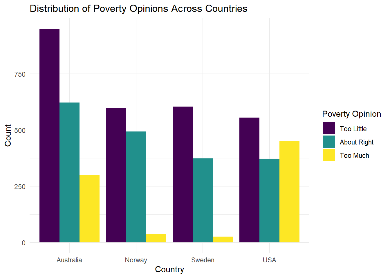

Question 9

Recreate the following visualization:

Show Answer

wvs |> 
    ggplot(aes(x = country, fill = degree)) +
    geom_bar(position = "fill") +
    labs(title = "Proportion of Degree Status by Country", 
       x = "Country", y = "Count", fill = "Degree Status") +
    theme_minimal()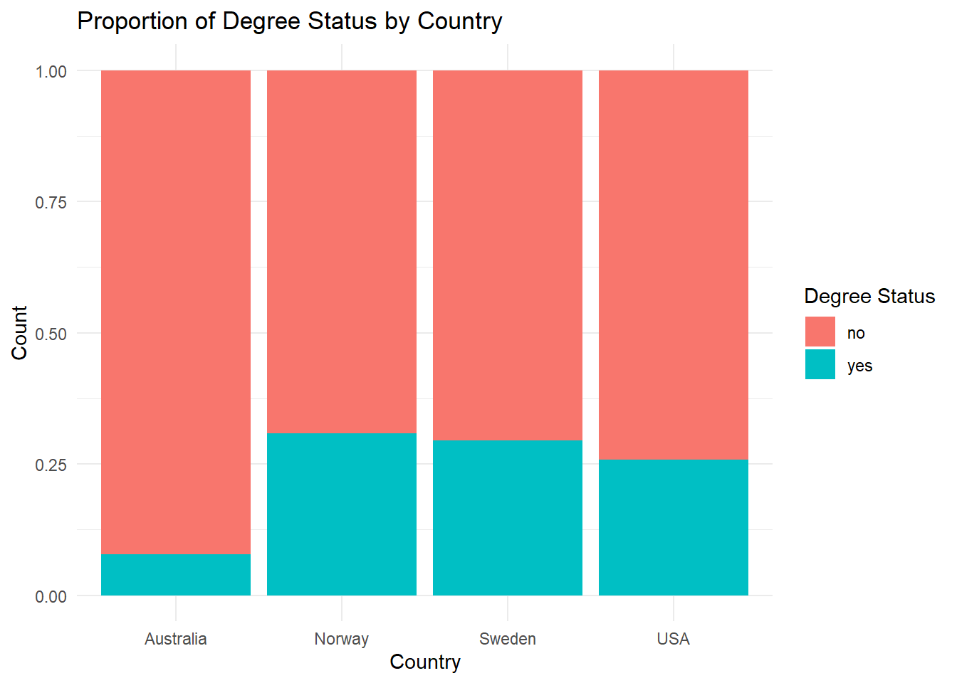

Question 10

Recreate the following visualization:

Show Answer

wvs |> ggplot(aes(x = country, y = age)) +
    geom_boxplot() +
    labs(title = "Age Distribution by Country", x = "Country", y = "Age") +
    theme_minimal() +
    theme(legend.position = "none")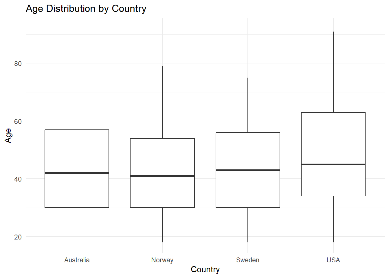

Question 11

Recreate the following visualization:

Show Answer

wvs |> 
    ggplot(aes(x = country, y = age)) +
    geom_boxplot() +
    facet_wrap(~ religion) +
    labs(title = "Age Distribution by Country and Religion",
       x = "Country", y = "Age") +
    theme_minimal()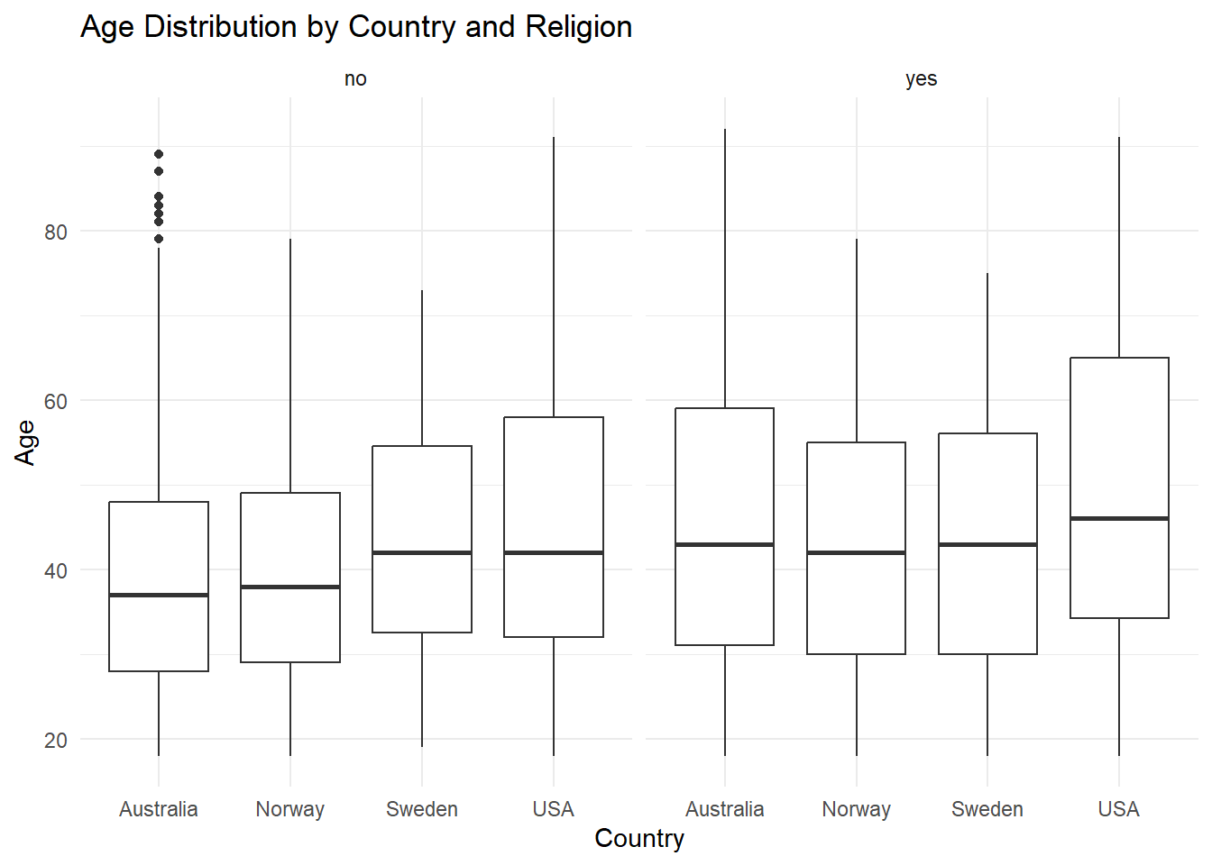

Question 12

Recreate the following visualization using duncan dataset:

Show Answer

duncan |> 
    ggplot(aes(x = income, y = prestige, color = type)) +
    geom_jitter() +
    labs(title = "Occupation Prestige vs. Income",
       x = "Income", 
       y = "Prestige Score",
       color = "Occupation Type") +
    theme_minimal()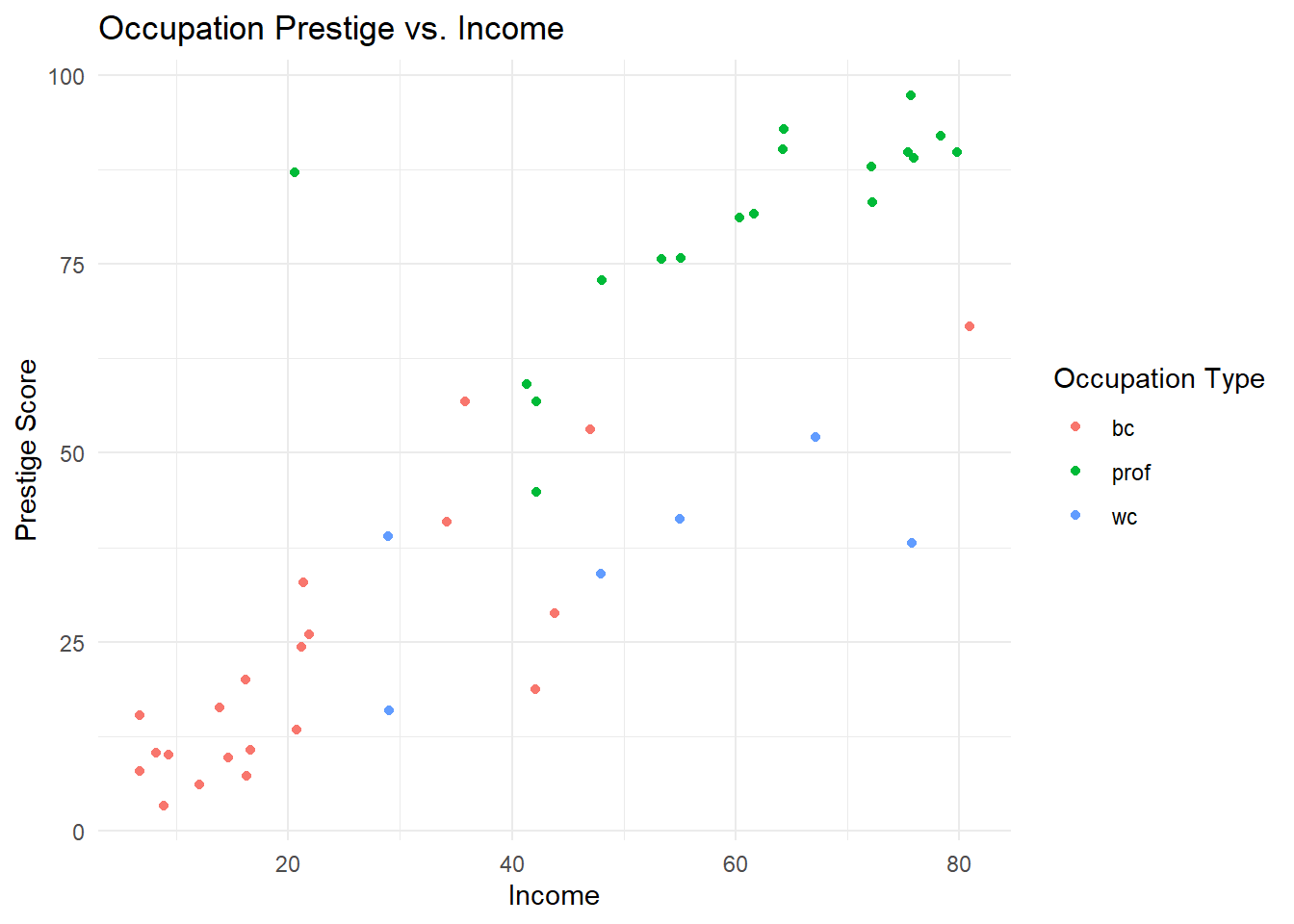

Question 13

Recreate the following visualization using duncan dataset:

Show Answer

duncan |> 
    ggplot(aes(x = type, y = income)) +
    geom_boxplot() +
    labs(title = "Income Distribution by Occupation Type",
        x = "Occupation Type",
        y = "Income") +
    theme_minimal()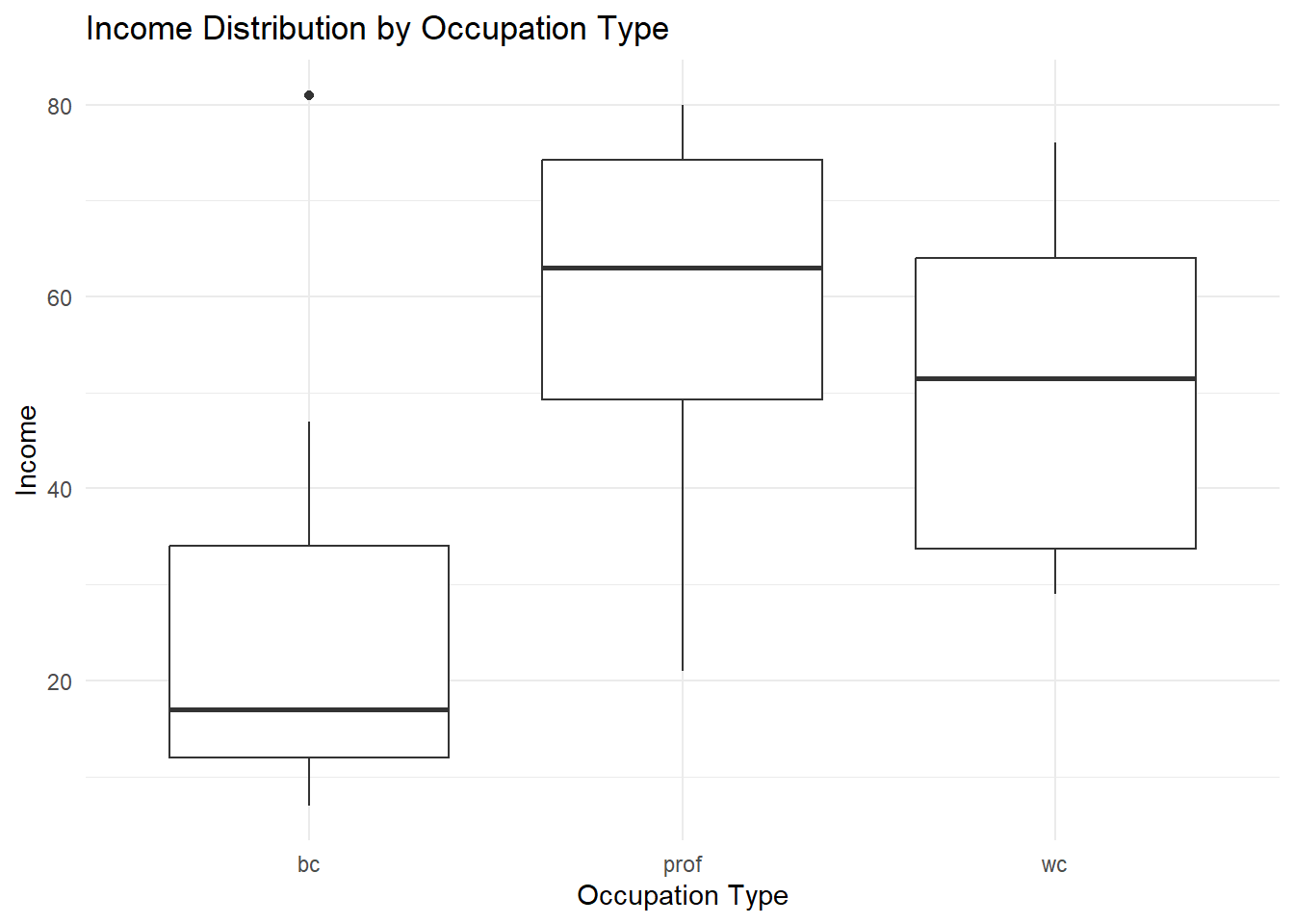

Question 14

Recreate the following visualization using duncan dataset:

Show Answer

duncan |> 
    ggplot(aes(x = prestige, y = income, color = type)) +
    geom_jitter() +
    geom_smooth(method = "lm") +
    labs(
        title = "Relationship between Prestige and Income",
        subtitle = "Grouped by Occupation Type",
        x = "Prestige Score",
        y = "Income",
        color = "Occupation Type"
    ) + 
    theme_minimal()

`geom_smooth()` using formula = 'y ~ x'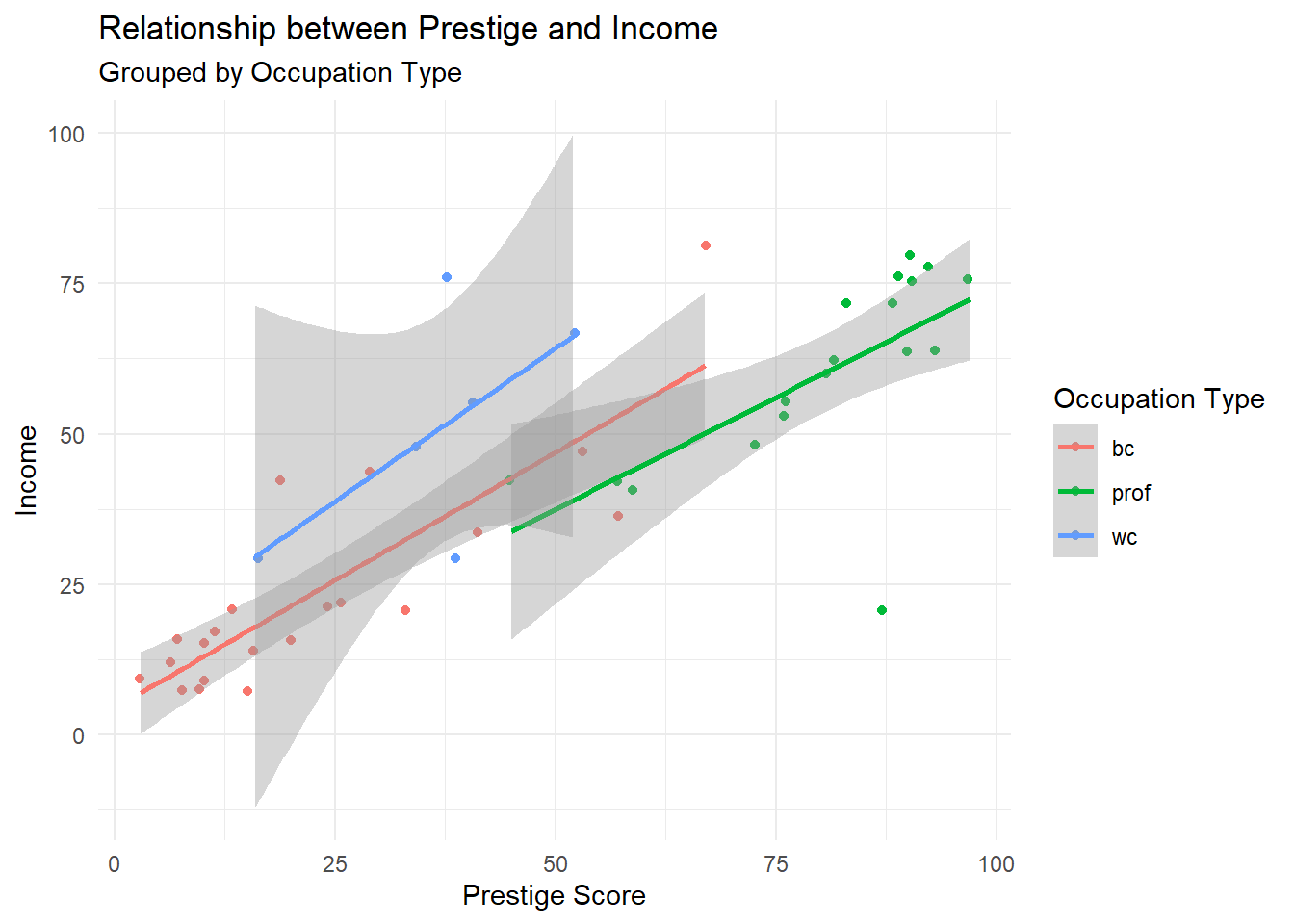

Question 15

Using duncan dataset:

Examine the correlation between prestige scores and education.
Analyze the relationship between income and prestige scores.

Show Answer

cor.test(duncan$prestige, duncan$education)


    Pearson's product-moment correlation

data:  duncan$prestige and duncan$education
t = 10.668, df = 43, p-value = 1.171e-13
alternative hypothesis: true correlation is not equal to 0
95 percent confidence interval:
 0.7445746 0.9163112
sample estimates:
      cor 
0.8519156

Show Answer

cor.test(duncan$prestige, duncan$income)


    Pearson's product-moment correlation

data:  duncan$prestige and duncan$income
t = 10.062, df = 43, p-value = 7.144e-13
alternative hypothesis: true correlation is not equal to 0
95 percent confidence interval:
 0.7217665 0.9080298
sample estimates:
      cor 
0.8378014

Question 16

Using duncan dataset, compare prestige scores across different occupational categories using ANOVA.

Show Answer

duncan_anova <- aov(prestige ~ type, data=duncan)
summary(duncan_anova)

            Df Sum Sq Mean Sq F value   Pr(>F)    
type         2  33090   16545   65.57 1.21e-13 ***
Residuals   42  10598     252                     
---
Signif. codes:  0 '***' 0.001 '**' 0.01 '*' 0.05 '.' 0.1 ' ' 1

Question 17

Using duncan dataset, create a regression model that predicts income based on occupational prestige and education scores.

library(huxtable)

Show Answer

duncan_model <- lm(income ~ prestige + education, data = duncan)
huxreg("income" = duncan_model)

	income
(Intercept)	10.426 *
	(4.164)
prestige	0.624 ***
	(0.125)
education	0.032
	(0.132)
N	45
R2	0.702
logLik	-179.902
AIC	367.805
* p < 0.001; p < 0.01; * p < 0.05.

Question 18

Using the wvs dataset, examine the relationship between religion and poverty perception.

Show Answer

wvs_chisq <- chisq.test(table(wvs$religion, wvs$poverty))
print(wvs_chisq)


    Pearson's Chi-squared test

data:  table(wvs$religion, wvs$poverty)
X-squared = 0.083005, df = 2, p-value = 0.9593

Question 19

Using the wvs dataset, examine whether there is a significant difference in the average age between individuals with and without a university degree.

Show Answer

wvs_ttest <- t.test(age ~ degree, data = wvs)
print(wvs_ttest)


    Welch Two Sample t-test

data:  age by degree
t = 7.0571, df = 2029, p-value = 2.325e-12
alternative hypothesis: true difference in means between group no and group yes is not equal to 0
95 percent confidence interval:
 2.674321 4.732708
sample estimates:
 mean in group no mean in group yes 
         45.82775          42.12423

Question 20

Using wvs dataset, compare the mean of age across different countries and age categories (see Question 7 to create age_category), and investigate if there is any significant difference. Conduct the post-hoc test if needed.

Show Answer

wvs_anova <- aov(age ~ country + age_category, data = wvs)
summary(wvs_anova)

               Df  Sum Sq Mean Sq F value Pr(>F)    
country         3   17399    5800   235.9 <2e-16 ***
age_category    3 1424858  474953 19319.9 <2e-16 ***
Residuals    5374  132113      25                   
---
Signif. codes:  0 '***' 0.001 '**' 0.01 '*' 0.05 '.' 0.1 ' ' 1