Introduction to Pandas and Seaborn

Bella Ratmelia

Recap from yesterday

Python libraries / packages
Introduction to Numpy (+ numpy-financial)
Getting started with visualizations with matplotlib

Overview for today

Today, we will cover the typical steps when doing data analysis projects. For this session, we will do simple time series analysis.

Step 1: Loading and pre-processing data (with pandas)
Step 2: Time Series analysis
Step 3: Data Visualization (with Seaborn)

Step 1: Loading and pre-processing data (with pandas)

What’s Pandas?

pandas is a fast, powerful, flexible and easy to use open source data analysis and manipulation tool, built on top of the Python programming language. pandas aims to be the fundamental high-level building block for doing practical, real world data analysis in Python. ¹

Well-established Python library for data manipulation and analysis
Built on top of NumPy. Unlike Numpy who can be difficult to “read”, Dataframe presents data in tabular format that’s easier for humans to read and perceive.
Provides DataFrame and Series data structures
Many cheatsheets available: https://pandas.pydata.org/Pandas_Cheat_Sheet.pdf or https://python-graph-gallery.com/cheat-sheets/

Comparison to Numpy

Feature	NumPy Array	pandas DataFrame
Data Types	All elements must be of the same type (e.g., integers, floats).	Different columns can hold different data types (e.g., integers, floats, strings).
Performance	Faster for numerical computations due to homogeneity and optimized implementation.	Slightly slower but more flexible for working with heterogeneous or labeled data.
Dimensionality	Can be multi-dimensional (1D, 2D, 3D, etc.).	Always two-dimensional with labeled rows and columns.
Indexing	Purely positional indexing (e.g., `array[0, 1]`).	Labeled-based indexing (`loc`), position-based indexing (`iloc`), access by both labels and positions.
Usage	Primarily for high-performance numerical and scientific computations.	Primarily for data manipulation, analysis, and cleaning, especially for tabular and real-world datasets.

Installing and importing packages

To install this package, you can use this command:

pip install pandas

pip install seaborn

Remember, we must first import these packages to our notebook / script before we can use them.

import pandas as pd
import matplotlib.pyplot as plt
import seaborn as sns

Pandas Cheatsheet

Have this cheatsheet open on another tab as you work through your data: https://pandas.pydata.org/Pandas_Cheat_Sheet.pdf or https://python-graph-gallery.com/cheat-sheets/

Load data from CSV to DataFrame

Before we begin…

Right-click here to open unemployment-age.csv, and then Ctrl + S / Cmd + S to save it locally into your data folder

Typically, we load the data from API source (more on this next week!) or external data file such as CSV. Let’s load the unemployment-age.csv now!

unemp_data = pd.read_csv('data/unemployment-age.csv')
print(unemp_data.head())

         date  16_19yrs  20_24yrs  25_54yrs  55yrs_onwards  Unnamed: 5
0  1948-01-01      10.1       6.6       3.0            3.6         NaN
1  1948-02-01      11.5       8.0       3.6            4.0         NaN
2  1948-03-01      10.8       8.6       3.2            3.5         NaN
3  1948-04-01       8.8       6.8       3.2            3.2         NaN
4  1948-05-01       6.9       6.3       2.6            2.9         NaN

Initial checks: get basic info

The first thing that you should always do is check on the dataframe to get an overview of it. The function info() will tell us the data types for each columns, the number of observations, and index info if there’s any.

unemp_data.info()

<class 'pandas.core.frame.DataFrame'>
RangeIndex: 920 entries, 0 to 919
Data columns (total 6 columns):
 #   Column         Non-Null Count  Dtype  
---  ------         --------------  -----  
 0   date           920 non-null    object 
 1   16_19yrs       920 non-null    float64
 2   20_24yrs       920 non-null    float64
 3   25_54yrs       920 non-null    float64
 4   55yrs_onwards  920 non-null    float64
 5   Unnamed: 5     0 non-null      float64
dtypes: float64(5), object(1)
memory usage: 43.3+ KB

Initial checks: get summary stats

Also get the summary statistics to get a sense of the shape and spread of your data.

unemp_data.describe()

	16_19yrs	20_24yrs	25_54yrs	55yrs_onwards	Unnamed: 5
count	920.000000	920.000000	920.000000	920.00000	0.0
mean	15.913370	9.259674	4.560109	3.79837	NaN
std	4.270376	2.790013	1.585635	1.23832	NaN
min	5.700000	3.300000	1.800000	1.50000	NaN
25%	13.000000	7.575000	3.400000	2.90000	NaN
50%	15.600000	8.900000	4.300000	3.50000	NaN
75%	18.400000	10.700000	5.500000	4.40000	NaN
max	32.200000	25.000000	12.600000	13.40000	NaN

Initial checks: column names

Optional, but you may also want to check on the column names to see how it appears in our environment (useful if you happen to have non UTF-8 characters as your column names)

print(unemp_data.columns)

Index(['date', '16_19yrs', '20_24yrs', '25_54yrs', '55yrs_onwards',
       'Unnamed: 5'],
      dtype='object')

Dropping columns

In some cases, we don’t really need the entire columns. Let’s drop the last column (that looks like an error in the CSV formatting).

unemp_data.drop(unemp_data.columns[-1], axis = 1, inplace= True)
unemp_data.head()

	date	16_19yrs	20_24yrs	25_54yrs	55yrs_onwards
0	1948-01-01	10.1	6.6	3.0	3.6
1	1948-02-01	11.5	8.0	3.6	4.0
2	1948-03-01	10.8	8.6	3.2	3.5
3	1948-04-01	8.8	6.8	3.2	3.2
4	1948-05-01	6.9	6.3	2.6	2.9

Renaming columns

Sometimes the column names are not ideal. In our case, let’s give a name to each age group!

unemp_data.columns = ['date', 'teenagers', 'young_adults', 'adults', 'seniors']
print(unemp_data.columns)

Index(['date', 'teenagers', 'young_adults', 'adults', 'seniors'], dtype='object')

Alternatively, if you just want to rename specific columns:

unemp_data.rename(columns={'16_19yrs': 'teenagers', '20_24yrs': 'young_adults'}, inplace = True)

Data preparation, analysis, and visualization tasks

Data preparation, analysis, and visualization tasks will be different depends on the dataset and your goal. Specifically for our data, we will do the following:

Check for and remove all the missing values.
We are primarily interested in the young adult unemployment. Separate this data into a new dataframe called ya_unemp.
Retrieve the months and years where the young adult rate is more than 10 percent and keep this on high_ya_unemp.
Add in a new column that tracks the total unemployment rate for each month.
Calculate the quarterly mean unemployment rate.
Calculate the year-on-year change of unemployment rate.
Plot the unemployment rate over the years for each age group.
Are there any specific month where the unemployment rate tends to be higher? Plot the data.
Are there any outliers in the unemployment rate?

Task 1 - Handling missing values

Other than info(), we can also use isnull() to check for null values

# Check for missing values
print(unemp_data.isnull().sum())

date            0
teenagers       0
young_adults    0
adults          0
seniors         0
dtype: int64

Handling missing values: drop or no drop?

We can drop those rows that contains null values with dropna()…

# Drop rows with missing values (if any)
unemp_data = unemp_data.dropna()
print(unemp_data.info())

<class 'pandas.core.frame.DataFrame'>
RangeIndex: 920 entries, 0 to 919
Data columns (total 5 columns):
 #   Column        Non-Null Count  Dtype  
---  ------        --------------  -----  
 0   date          920 non-null    object 
 1   teenagers     920 non-null    float64
 2   young_adults  920 non-null    float64
 3   adults        920 non-null    float64
 4   seniors       920 non-null    float64
dtypes: float64(4), object(1)
memory usage: 36.1+ KB
None

… or we can also fill in the null values with something else, e.g. 0

uemp_data = unemp_data.fillna(0)

Task 2 - Retrieving columns: a single column

As the column names in DataFrame are indexed, we can simply call them by their column names! (Much more intuitive compared to Numpy)

ya_unemp = unemp_data['young_adults']
ya_unemp.head()

0    6.6
1    8.0
2    8.6
3    6.8
4    6.3
Name: young_adults, dtype: float64

Retrieving columns: multiple columns

Similarly, if we want to retrieve multiple columns, we can pass a list of column names to the dataframe and save these sliced columns into a new dataframe.

ya_unemp = unemp_data[['date', 'young_adults']]
ya_unemp.head()

	date	young_adults
0	1948-01-01	6.6
1	1948-02-01	8.0
2	1948-03-01	8.6
3	1948-04-01	6.8
4	1948-05-01	6.3

Task 3 - Filtering row(s): without query()

We can do it “raw” or us the query function from pandas. Here is how you can do it without the query() function:

criteria = unemp_data["young_adults"] > 10
high_ya_unemp = unemp_data[criteria]
high_ya_unemp.head()

	date	teenagers	young_adults	adults	seniors
17	1949-06-01	19.0	10.1	4.4	4.9
18	1949-07-01	16.0	11.2	5.3	5.8
19	1949-08-01	12.6	10.4	5.0	5.3
24	1950-01-01	17.7	11.6	6.2	6.6
25	1950-02-01	17.3	12.2	6.4	7.0

Filtering row(s): with query()

And here is how you can do it with the query() function:

print(unemp_data.query('young_adults > 10'))

           date  teenagers  young_adults  adults  seniors
17   1949-06-01       19.0          10.1     4.4      4.9
18   1949-07-01       16.0          11.2     5.3      5.8
19   1949-08-01       12.6          10.4     5.0      5.3
24   1950-01-01       17.7          11.6     6.2      6.6
25   1950-02-01       17.3          12.2     6.4      7.0
..          ...        ...           ...     ...      ...
873  2020-10-01       13.1          10.5     6.2      5.2
875  2020-12-01       14.1          10.6     5.7      5.8
876  2021-01-01       15.6          10.8     6.2      5.6
878  2021-03-01       12.5          10.4     5.7      4.8
880  2021-05-01        9.5          10.3     4.9      4.6

[311 rows x 5 columns]

Filtering row(s): with query() and save result

Take note that the previous code will simply print out the result! If you want to save the result, make sure to assign the result to a new dataframe.

high_ya_unemp = unemp_data.query('young_adults > 10')
high_ya_unemp.head()

	date	teenagers	young_adults	adults	seniors
17	1949-06-01	19.0	10.1	4.4	4.9
18	1949-07-01	16.0	11.2	5.3	5.8
19	1949-08-01	12.6	10.4	5.0	5.3
24	1950-01-01	17.7	11.6	6.2	6.6
25	1950-02-01	17.3	12.2	6.4	7.0

Task 4 - Adding new column(s)

Let’s add a new column for total unemployment (sum of all age groups)

unemp_data['total_unemployment'] = unemp_data['teenagers'] + unemp_data['young_adults'] + unemp_data['adults'] + unemp_data['seniors']
unemp_data.head()

	date	teenagers	young_adults	adults	seniors	total_unemployment
0	1948-01-01	10.1	6.6	3.0	3.6	23.3
1	1948-02-01	11.5	8.0	3.6	4.0	27.1
2	1948-03-01	10.8	8.6	3.2	3.5	26.1
3	1948-04-01	8.8	6.8	3.2	3.2	22.0
4	1948-05-01	6.9	6.3	2.6	2.9	18.7

Learning Check #1

Retrieve data where the employment rate for adults are between 9 to 12 inclusive. Save only the date and adults column to a new dataframe called adult_unemp

Code

adult_unemp = unemp_data[['date', 'adults']].query('adults >= 9 & adults <= 12')
print(adult_unemp.head())
print(adult_unemp.shape)

           date  adults
419  1982-12-01     9.0
420  1983-01-01     9.7
421  1983-02-01     9.6
422  1983-03-01     9.2
744  2010-01-01     9.6
(10, 2)

Step 2: Time Series Analysis

Side quest: DateTime Object

A DateTime object in Python, provided by the datetime module, represents a specific point in time, including the year, month, day, hour, minute, second, and microsecond.
It can be used to manipulate dates and times, perform arithmetic on dates, and format dates into other string representation e.g. from dd/mm/yyyy to yyyy-mm-dd.

from datetime import datetime

now = datetime.now()
print("Current Date and Time:", now)

Current Date and Time: 2024-10-10 16:36:39.130939

Components of DateTime

The DateTime object consists of multiple components that represent different parts of the date and time, such as year, month, day, hour, minute, second, etc. You can access these components individually.

# Extract year, month, and day from a specific date
now = datetime.now()

# Access individual components
print("Year:", now.year)
print("Month:", now.month)
print("Day:", now.day)
print("Hour:", now.hour)
print("Minute:", now.minute)
print("Second:", now.second)

Year: 2024
Month: 10
Day: 10
Hour: 16
Minute: 36
Second: 39

DateTime operations

You can perform various operations with DateTime objects, such as calculating the difference between two dates or adding/subtracting time with the help of timedelta.
These are essential for time series data manipulation, where date-based arithmetic is often required.

from datetime import timedelta

now = datetime.now()

last_week = now - timedelta(days=7)
print("1 week ago:", last_week)

1 week ago: 2024-10-03 16:36:39.164502

Back to Main Quest: Time Series with DataFrame

Let’s index the rows under date column as a DateTime index.

1unemp_data['date'] = pd.to_datetime(unemp_data['date'], format="%Y-%m-%d")
2unemp_data.set_index('date', inplace=True)

1: Convert the data type under date column from string to DateTime object
2: Set the date column as the index.

DateTime is the index, now what?

Let’s check on the dataframe once more, to make sure that it is indexed as intended:

unemp_data.info()

<class 'pandas.core.frame.DataFrame'>
DatetimeIndex: 920 entries, 1948-01-01 to 2024-08-01
Data columns (total 5 columns):
 #   Column              Non-Null Count  Dtype  
---  ------              --------------  -----  
 0   teenagers           920 non-null    float64
 1   young_adults        920 non-null    float64
 2   adults              920 non-null    float64
 3   seniors             920 non-null    float64
 4   total_unemployment  920 non-null    float64
dtypes: float64(5)
memory usage: 43.1 KB

If all goes well, the date column should be part of the index now.

Extra checks with Time Series

Other things that we may want to check with Time Series is the date range of our data.

print("start date", unemp_data.index.min())
print("end date", unemp_data.index.max())
print("length", unemp_data.index.max() - unemp_data.index.min())

start date 1948-01-01 00:00:00
end date 2024-08-01 00:00:00
length 27972 days 00:00:00

Retrieve specific date range

Now that the index is a DateTime object, we can easily retrieve specific date range! Let’s say we would like retrieve unemployment rate for during COVID, which will be March 2020 to May 2023.

unemp_data_covid = unemp_data.loc['2020-03':'2023-05']
print(unemp_data_covid.head())

            teenagers  young_adults  adults  seniors  total_unemployment
date                                                                    
2020-03-01       13.7           8.6     3.9      3.5                29.7
2020-04-01       32.2          25.0    12.6     13.4                83.2
2020-05-01       30.7          23.2    11.2     11.5                76.6
2020-06-01       24.5          20.1     9.7      9.7                64.0
2020-07-01       19.1          18.2     9.3      9.0                55.6

Task 5 - Resampling to Quarterly data and get the quarterly mean

With time series, we can calculate the quarterly average based on the monthly data with resample()

quarterly_data = unemp_data.resample('Q').mean()
print(quarterly_data.head())

            teenagers  young_adults    adults   seniors  total_unemployment
date                                                                       
1948-03-31  10.800000      7.733333  3.266667  3.700000           25.500000
1948-06-30   9.700000      6.466667  2.733333  2.900000           21.800000
1948-09-30   8.933333      5.500000  2.766667  2.700000           19.900000
1948-12-31   7.066667      4.933333  2.600000  3.166667           17.766667
1949-03-31  12.033333      8.700000  4.366667  5.000000           30.100000

Resampling to Yearly data

Let’s find out what is the highest unemployment rate for each year!

yearly_data = unemp_data.resample('Y').max()
print(yearly_data.head())

            teenagers  young_adults  adults  seniors  total_unemployment
date                                                                    
1948-12-31       13.4           8.6     3.6      4.0                27.1
1949-12-31       19.0          11.2     5.3      5.8                38.4
1950-12-31       17.7          12.2     6.4      7.0                42.9
1951-12-31       12.2           5.0     3.6      4.9                23.1
1952-12-31       12.2           5.4     3.2      3.4                21.7

Saving into a CSV

Let’s save the quarterly data to a CSV!

quarterly_data.to_csv("data-output/yearly-unemployment-age.csv")

Changing the frequency of Time Series: More granular

Let’s say we would like get a weekly time series. Since our data is a monthly one, there will be rows with empty values if we change the frequency. There are several methods that we can employ here to fill this empty values:

backfill
forward fill
interpolate

unemp_data_weekly = unemp_data.resample('1W').ffill()
print(unemp_data_weekly.tail())

            teenagers  young_adults  adults  seniors  total_unemployment
date                                                                    
2024-07-07       13.2           8.1     3.8      3.3                28.4
2024-07-14       13.2           8.1     3.8      3.3                28.4
2024-07-21       13.2           8.1     3.8      3.3                28.4
2024-07-28       13.2           8.1     3.8      3.3                28.4
2024-08-04       14.1           8.0     3.7      3.1                28.9

Task 6 - Calculate year-on-year changes for young adults

Let’s get the year-on-year change for young adults age group.

unemp_data['ya_YoY_pctchange'] = unemp_data['young_adults'].pct_change(periods=12) # multiply by 100 to get the %
print(unemp_data.tail())

            teenagers  young_adults  adults  seniors  total_unemployment  \
date                                                                       
2024-04-01       10.4           6.0     3.0      2.8                22.2   
2024-05-01       12.1           8.0     3.1      2.5                25.7   
2024-06-01       14.4           8.2     3.5      2.9                29.0   
2024-07-01       13.2           8.1     3.8      3.3                28.4   
2024-08-01       14.1           8.0     3.7      3.1                28.9   

            ya_YoY_pctchange  
date                          
2024-04-01          0.250000  
2024-05-01          0.269841  
2024-06-01          0.223881  
2024-07-01          0.125000  
2024-08-01          0.111111

Calculate the changes for each month

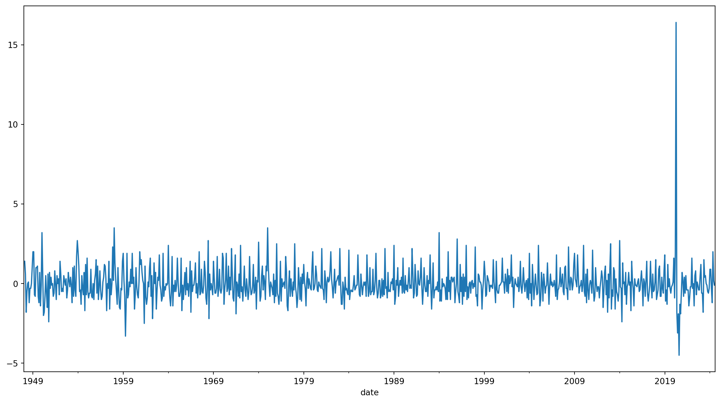
To capture the direction and magnitude of changes in unemployment rate each month, use diff() function.

unemp_data['changes_ya'] = unemp_data['young_adults'].diff()
print(unemp_data['changes_ya'].head(7))

date
1948-01-01    NaN
1948-02-01    1.4
1948-03-01    0.6
1948-04-01   -1.8
1948-05-01   -0.5
1948-06-01    0.0
1948-07-01    0.1
Name: changes_ya, dtype: float64

Visualize the changes

Pandas is built on top of NumPy and integrates well with Matplotlib, so it is super easy to plot data right away—especially now that we’ve set the index!

unemp_data['changes_ya'].plot()

Learning Check #2

Change the frequency of the time series to weekly, and interpolate the numbers. Save this new series into unemp_weekly_interpolate

Code

unemp_weekly_interpolate = unemp_data.resample('1W').interpolate()
print(unemp_weekly_interpolate.tail())

            teenagers  young_adults  adults  seniors  total_unemployment  \
date                                                                       
2024-07-07       13.1           6.6     3.0      2.5                25.2   
2024-07-14       13.1           6.6     3.0      2.5                25.2   
2024-07-21       13.1           6.6     3.0      2.5                25.2   
2024-07-28       13.1           6.6     3.0      2.5                25.2   
2024-08-04       13.1           6.6     3.0      2.5                25.2   

            ya_YoY_pctchange  changes_ya  
date                                      
2024-07-07          0.015385        -0.5  
2024-07-14          0.015385        -0.5  
2024-07-21          0.015385        -0.5  
2024-07-28          0.015385        -0.5  
2024-08-04          0.015385        -0.5

Step 3: Data visualization

What’s Seaborn?

Seaborn is a Python data visualization library based on matplotlib. It provides a high-level interface for drawing attractive and informative statistical graphics. ¹

Well-established Python library for data visualization
Cheatsheet by Datacamp here: https://python-graph-gallery.com/cheat-sheets/

Some setups we can do:

import seaborn as sns
sns.set_style("whitegrid")
sns.set_palette("husl")

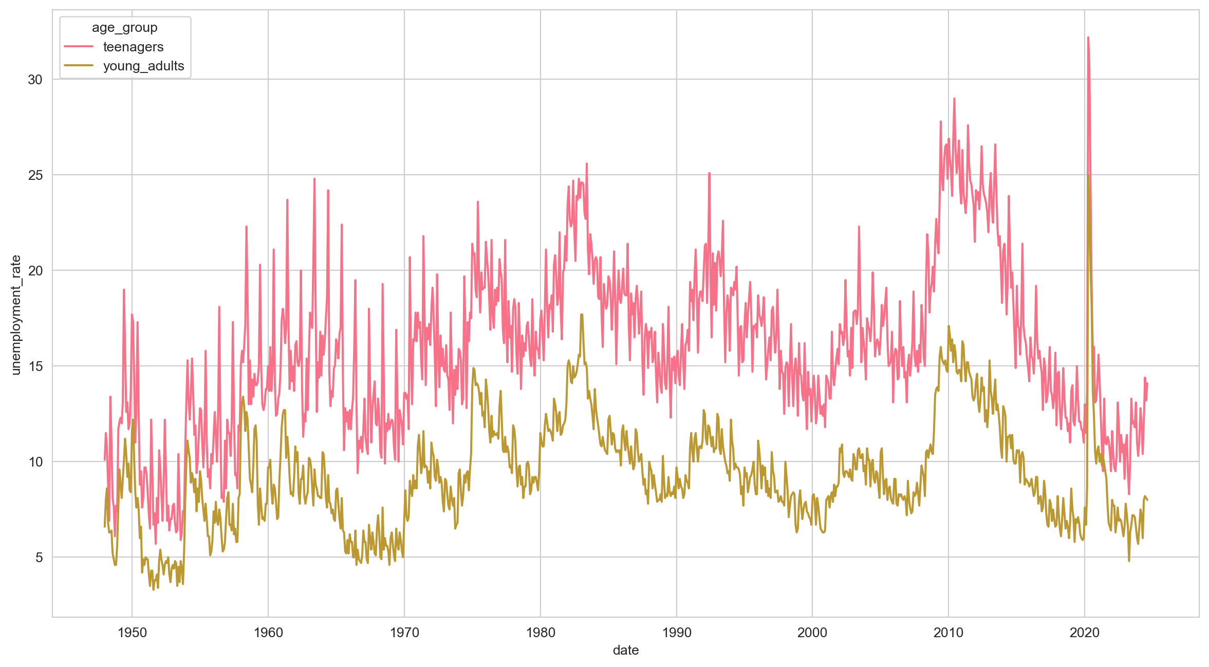
Task 7 - Plot the entire time series

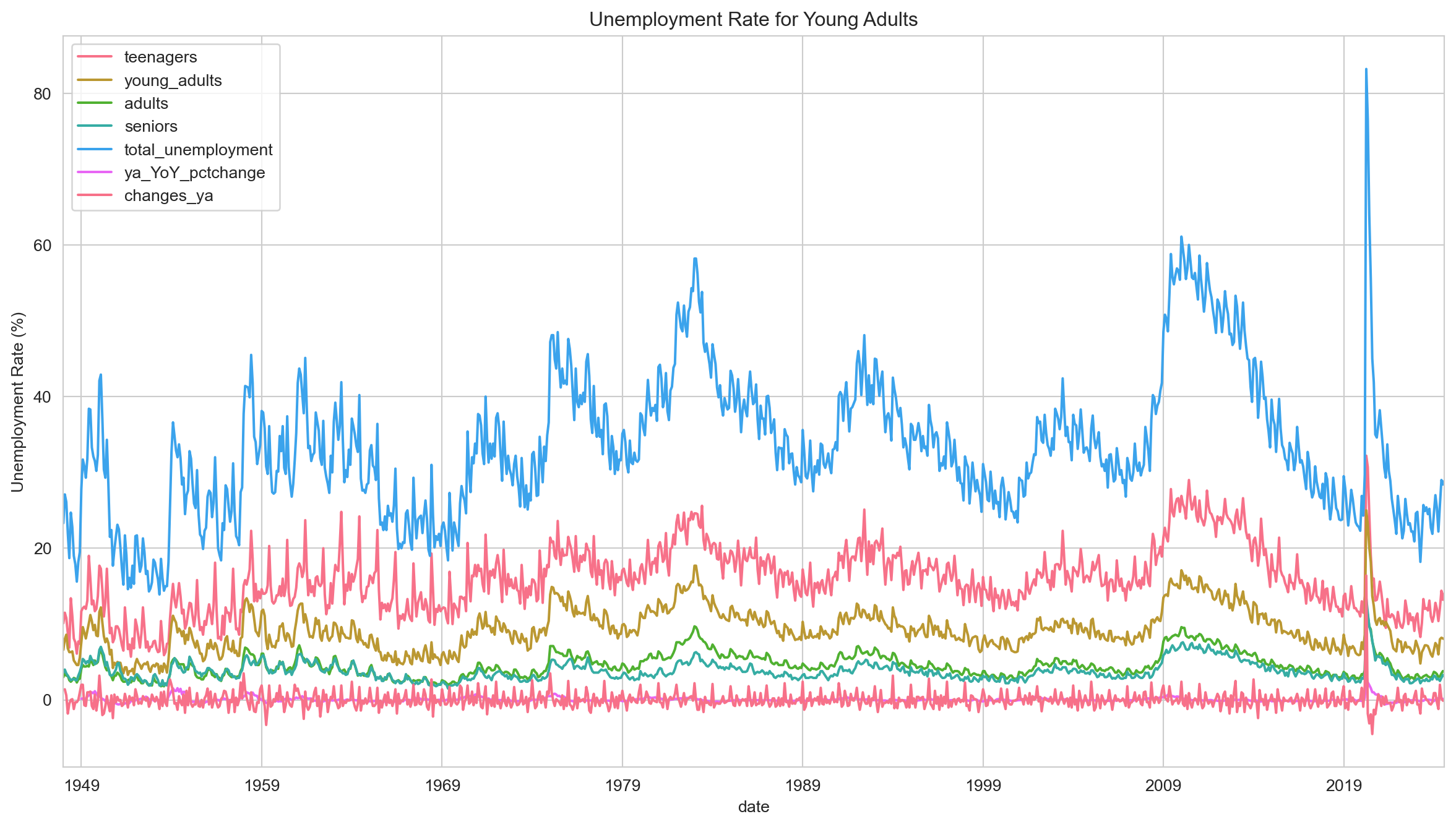
Let’s plot the unemployment rate over the years for each age group!

unemp_data.plot()
plt.title('Unemployment Rate for Young Adults')
plt.ylabel('Unemployment Rate (%)')
plt.show()

Task 7 - Plot the entire time series

Plotting some parts of the time series

Clearly, there are some columns that we may want to skip. To do this, we can reshape the data shape into long format using melt().

Let’s say we only want to visualize teenagers and young_adults.

1youth_data = unemp_data[['teenagers', 'young_adults']]
2youth_data = youth_data.reset_index()
3youth_data_melted = youth_data.melt(id_vars='date', value_vars=['teenagers', 'young_adults'], var_name='age_group', value_name='unemployment_rate')

1: Retrieve the columns that we need (index will be automatically included)
2: Reset the index, so that it’s back to normal column.
3: Use the melt() function to “melt” the wide data into long format

Wide data vs Long data

Check out the difference!

Wide Data

            teenagers  young_adults
date                               
1948-01-01       10.1           6.6
1948-02-01       11.5           8.0
1948-03-01       10.8           8.6
1948-04-01        8.8           6.8
1948-05-01        6.9           6.3
...               ...           ...
2024-04-01       10.4           6.0
2024-05-01       12.1           8.0
2024-06-01       14.4           8.2
2024-07-01       13.2           8.1
2024-08-01       14.1           8.0

[920 rows x 2 columns]

Long Data

           date     age_group  unemployment_rate
0    1948-01-01     teenagers               10.1
1    1948-02-01     teenagers               11.5
2    1948-03-01     teenagers               10.8
3    1948-04-01     teenagers                8.8
4    1948-05-01     teenagers                6.9
...         ...           ...                ...
1835 2024-04-01  young_adults                6.0
1836 2024-05-01  young_adults                8.0
1837 2024-06-01  young_adults                8.2
1838 2024-07-01  young_adults                8.1
1839 2024-08-01  young_adults                8.0

[1840 rows x 3 columns]

Visualizing is much easier with long data

We can now fit the things we want in a single line like so:

sns.lineplot(data=youth_data_melted, x='date', y='unemployment_rate', hue='age_group')

Making visualization easier: Capture month info into a separate column

With DateTime object as the index, we can easily capture the month info. This would be useful to see whether certain months tend to have higher unemployment rate based on this data.

unemp_data['month'] = unemp_data.index.month
print(unemp_data.head())

            teenagers  young_adults  adults  seniors  total_unemployment  \
date                                                                       
1948-01-01       10.1           6.6     3.0      3.6                23.3   
1948-02-01       11.5           8.0     3.6      4.0                27.1   
1948-03-01       10.8           8.6     3.2      3.5                26.1   
1948-04-01        8.8           6.8     3.2      3.2                22.0   
1948-05-01        6.9           6.3     2.6      2.9                18.7   

            ya_YoY_pctchange  changes_ya  month  
date                                             
1948-01-01               NaN         NaN      1  
1948-02-01               NaN         1.4      2  
1948-03-01               NaN         0.6      3  
1948-04-01               NaN        -1.8      4  
1948-05-01               NaN        -0.5      5

Aggregate statistics

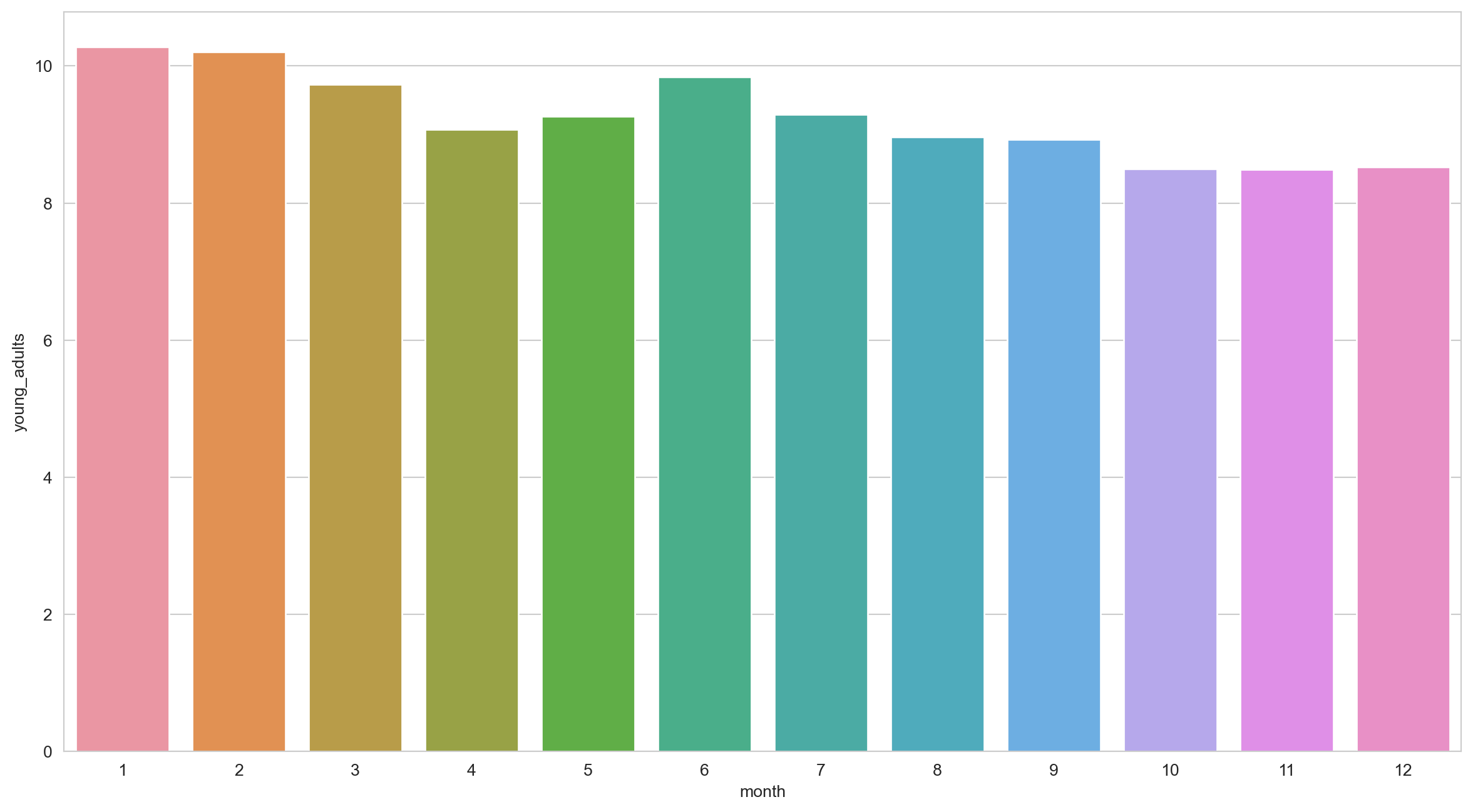
Let’s calculate the average unemployment rate for each month based on this data.

unemp_permonth = unemp_data.groupby('month').mean()
print(unemp_permonth)

       teenagers  young_adults    adults   seniors  total_unemployment  \
month                                                                    
1      16.612987     10.276623  5.159740  4.264935           36.314286   
2      16.648052     10.207792  5.135065  4.290909           36.281818   
3      15.977922      9.727273  4.905195  4.138961           34.749351   
4      15.248052      9.076623  4.589610  3.902597           32.816883   
5      15.981818      9.262338  4.322078  3.631169           33.197403   
6      19.632468      9.836364  4.367532  3.646753           37.483117   
7      16.216883      9.293506  4.528571  3.781818           33.820779   
8      14.025974      8.961039  4.501299  3.703896           31.192208   
9      15.543421      8.925000  4.292105  3.468421           32.228947   
10     15.027632      8.500000  4.178947  3.432895           31.139474   
11     15.502632      8.493421  4.297368  3.618421           31.911842   
12     14.502632      8.522368  4.430263  3.686842           31.142105   

       ya_YoY_pctchange  changes_ya  
month                                
1              0.023639    1.802632  
2              0.027765   -0.068831  
3              0.023718   -0.480519  
4              0.056689   -0.650649  
5              0.053468    0.185714  
6              0.040224    0.574026  
7              0.043577   -0.542857  
8              0.035135   -0.332468  
9              0.033654   -0.048684  
10             0.035276   -0.425000  
11             0.028284   -0.006579  
12             0.024550    0.028947

Task 8 - Months where unemployment rate then to be high

Which month seems to have the highest unemployment rate on average?

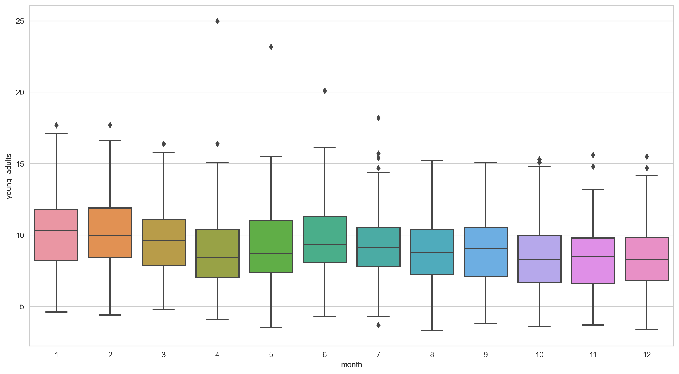
sns.barplot(data = unemp_permonth, x = unemp_permonth.index, y = 'young_adults')

Task 9 - Finding outliers

Let’s see how unemployment rate fared each month for young_adults. Are there any outliers?

sns.boxplot(x = 'month', y = 'young_adults', data=unemp_data[['month', 'young_adults']])

More Seaborn: Scatterplot

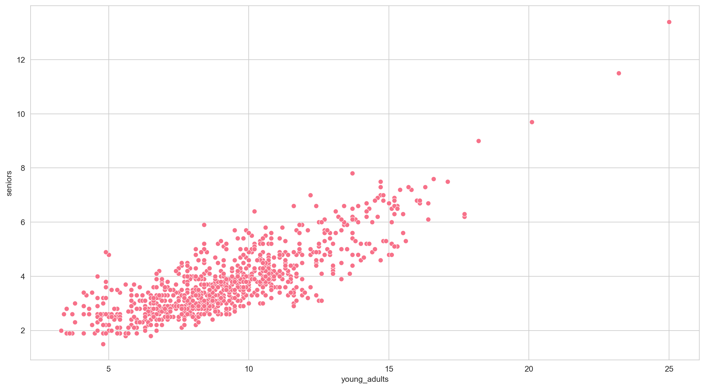
Seaborn can do many other visualizations as well. For example, let’s try plotting a scatterplot of young_adults and seniors

sns.scatterplot(x = 'young_adults', y = 'seniors', data = unemp_data)

More Seaborn: Regplot

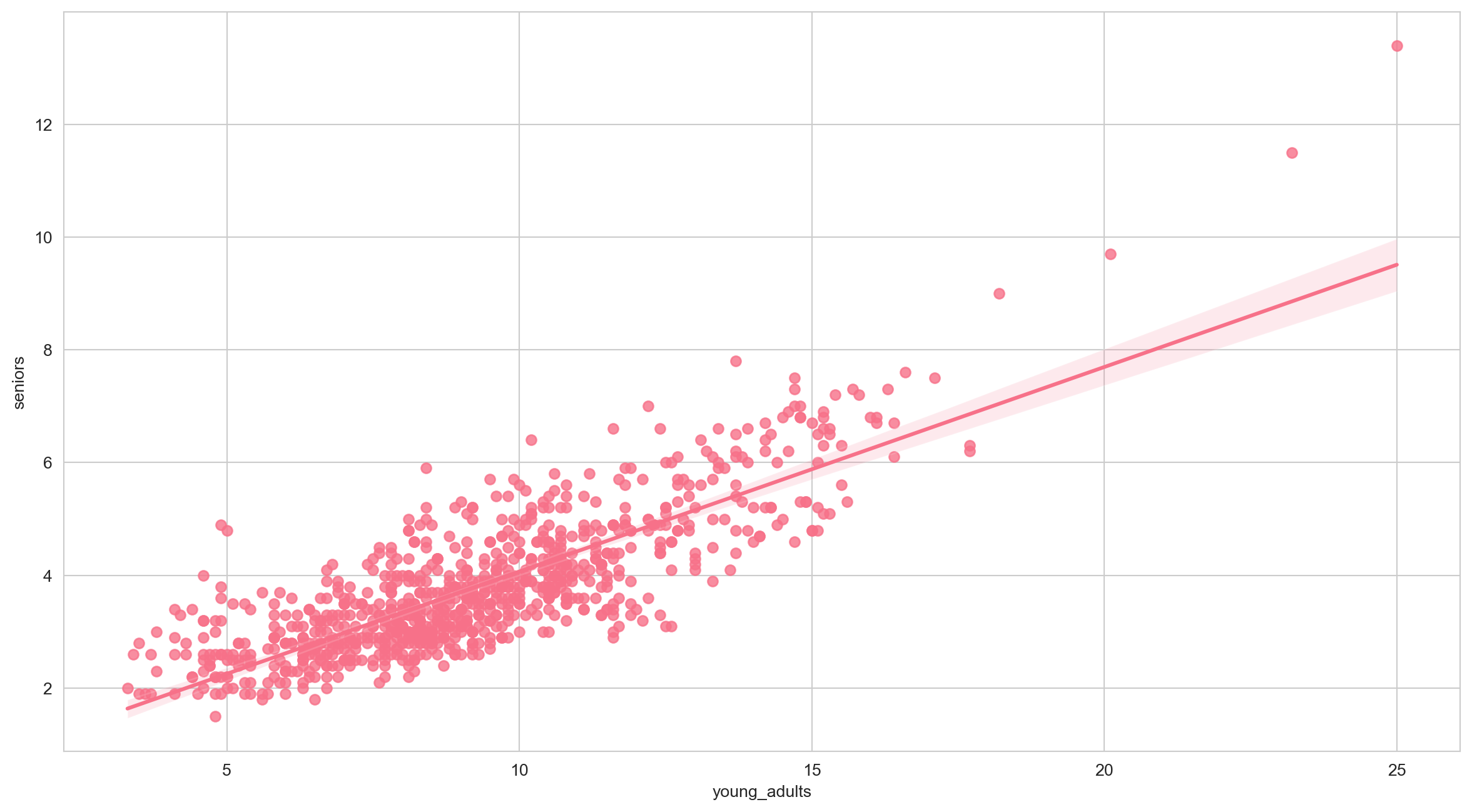
Let’s try plotting a regression plot of young_adults and seniors

sns.regplot(x = 'young_adults', y = 'seniors', data = unemp_data)

Learning Check #3

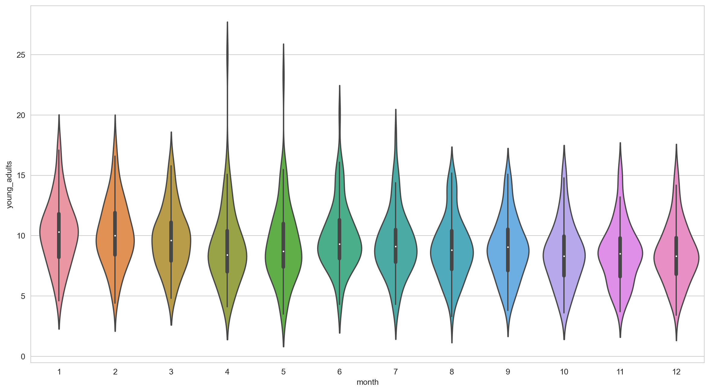
Plot the unemployment rate fared each month for young_adults with violin plot to see the distribution better.

Code

sns.violinplot(x = 'month', y = 'young_adults', data=unemp_data[['month', 'young_adults']])

End of Session 3!

We have covered pandas and Seaborn!